Hello World in Rust

After reading the paper from Google on Memory Safety, I decided to give Rust a try and do a simple Hello World: https://research.google/pubs/secure-by-design-googles-perspective-on-memory-safety/

Installation

It’s very simple, I installed Rust in Ubuntu by following this tutorial : How To Install Rust on Ubuntu 20.04 | DigitalOcean

The command to install is:

curl --proto '=https' --tlsv1.3 https://sh.rustup.rs -sSf | sh

After installing it, using Nano I created a testrust.rs file with the following contents:

fn main()
{
println!("Congratulations! Your Rust program works.");
}

Then, compiled it with the following command:

rustc test.rs -o testrs

To execute the binary:

./testrs

Congratulations! Your Rust program works!

Very easy!

Hello world in C++

I created a simple Hello World in C++ with the following contents:

#include <iostream>

int main()

{

std::cout << "Congratulations! Your C++ program works." << std::endl;

return 0;

}

Compiled the file with the following command:

g++ test.cpp -o testcpp

Simplified Comparison of C++ vs Rust

I decided to compare both in terms of source code size and binary size

ls -l

total 3728

-rw-rw-r-- 1 119 Mar 9 23:43 test.cpp

-rwxrwxr-x 1 17320 Mar 9 23:43 testcpp

-rw-rw-r-- 1 71 Mar 9 22:45 test.rs

-rwxrwxr-x 1 3785312 Mar 9 22:47 testrs

Source Code Size

The C++ File is 119 bytes where as the Rust file is only 71 bytes

C++ seems to be more verbose

Binary size

The C++ generated binary is only 17,320 bytes whereas the Rust binary is 3,785,312 bytes.

The Rust binary is significantly bigger
Amazon Machine Learning Solutions Lab

Amazon has a Machine Learning Solutions Lab that specializes in providing support to companies in developing AI algorithms to solve business challenges.

I got the opportunity to collaborate with them through Continental Automotive, they’re really bright and passionate Engineers.

To get more information on our collaboration please visit:

https://aws.amazon.com/blogs/machine-learning/achieve-in-vehicle-comfort-using-personalized-machine-learning-and-amazon-sagemaker/

Beaglebone Blue + Simulink Hello World!

Today I decided to play around with a Beaglebone Blue that I bought last week.
It’s very easy to bring it up:
1) I followed this guide: http://beagleboard.org/getting-started. I tried to install the drivers for Windows 10 but I couldn’t install them, it would keep failing, then on the same Getting Started guide says that it’s not necessary to install them if you’re using one of the latest builds.
2) After flashing an SD card with the latest Debian build, I powered up the board and my PC got an IP (192.168.7.1)
3) I logged in to the BBB via SSH, via a Web Browser and also via Cloud9. Cloud9 is a very cool IDE, it’s not super fast but it’s very useful, I can see myself using it moving forward.
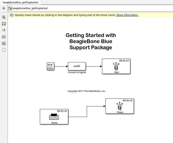
4) Since I’m a student at Georgia Tech, I got access to a free FULL License of MATLAB, so I decided to try Simulink. It’s actually very easy, I downloaded and installed the support package: https://www.mathworks.com/hardware-support/beaglebone-blue.html then ran and modified the GettingStarted simulink file (see image below).

Very simple to implement and to see running on the HW. The whole process took (from flashing a SD card to reading switch and controlling LEDs in Simulink) took less than 1hr.  I think I’m going to be having a lot of fun with the Beaglebone Blue! (They also have blocks to control motors!).

simulinkbbb

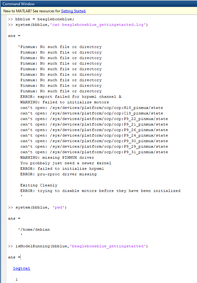
matlab_bbb

Expected Value in MATLAB

From Wikipedia:
“In probability theory, the expected value of a random variable, intuitively, is the long-run average value of repetitions of the experiment it represents.”

I decided to give it a try in MATLAB.

% Expected Value of a Die
numOfIterations = 100000;
meanArray = zeros([1 numOfIterations]);
values = zeros([1 numOfIterations]);

for i = 1:numOfIterations
   % Get a random value between the range of [1 6]
   values(i) = randi(6);
   % Calculate the mean so far
   meanArray(i) = mean(values(1:i));
end

%Plot
plot(1:numOfIterations, meanArray);

% Display the latest calculated mean
disp(meanArray(end));

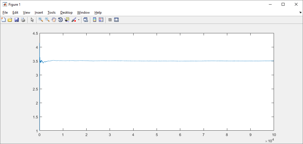
This is the result:

ExpectedValueMATLAB

OpenCV 3.4.1 + CUDA Hello World

The following code creates 3 floating-point matrices in RAM (imgA, imgB, imgC), and also 3 on the GPU (cuImgA, cuImgB, cuImgC).

Initializes imgA with 1.0 and imgB with 0.13. Then subtracts them using the GPU, copies the result from the GPU to RAM and displays the resultant image.

Hope this helps!


#include "iostream"
#include "opencv2/opencv.hpp"
#include "opencv2/imgproc.hpp"  // Gaussian Blur
#include "opencv2/videoio.hpp"
#include "opencv2/highgui.hpp"  // OpenCV window I/O

using namespace std;
using namespace cv;

int TEST_OpenCVCUDA()
{
	// Declare operands
	Mat imgA(Size(512, 512), CV_32F);
	Mat imgB(Size(512, 512), CV_32F);
	Mat imgC;

	cuda::GpuMat cuImgA, cuImgB, cuImgC;

	// Display information on the current environment setup
	cout << "CUDA Device count: \t" << cuda::getCudaEnabledDeviceCount() << endl;
	cout << "Cuda Device: " << cuda::getDevice() << endl;

	// Set the images to different values
	imgA = 1;
	imgB = 0.13;

	// Copy data from RAM to GPU
	cuImgA.upload(imgA);
	cuImgB.upload(imgB);

	// Perform arithmetic operation
	cuda::absdiff(cuImgA, cuImgB, cuImgC);

	// Download result to RAM from GPU
	cuImgC.download(imgC);

	cout << "Image A: " << imgA.at(255, 0) << endl;
	cout << "Image B: " << imgB.at(0, 255) << endl;
	cout << "Image C: " << imgC.at(255, 255) << endl;

	// Display image
	imshow("imgC", imgC);

	// Wait for a keystroke in the window
	waitKey(0);

	return 0;
}

int main()
{
	return TEST_OpenCVCUDA();
}

Building OpenCV 3.4.1 + CUDA

Requirements

  • CUDA Toolkit (I’m using version 9.1)
  • OpenCV (I’m using version 3.4.1)
  • CMake (I’m using version 3.10.1)
  • Visual Studio 2017

Process

Open CMake and selecte the sources folder as well as the folder where the build files will be generated (I created a folder named buildDATE).

Click on “Configure”, it will take sometime to configure everything, it may ask you to select the “Generator” (in this case select Visual Studio 15 2017 Win64).

Click on Generate.

Go to the build folder and open the OpenCV.sln file (the solution for Visual Studio).

Under CMakeTargets, right click on ALL_BUILD and Build. This will take a long time (it took over 2hrs in my case).

I  ran into a problem where the module/opencv_highgui was throwing linker errors, I had to manually add window_w32.cpp to the opencv_highgui project to get it to link correctly.

Verify that all the modules built correctly. Every module will generate a .lib and .dll file.

Under CMakeTargets, right click on INSTALL and build. This will take some time but not as much as the ALL_BUILD project. This will generate a folder named “install/x64/vc15” with 2 subfolders: “bin” and “lib”.

After this, you are ready to start developing with OpenCV 3.4.1 + CUDA, next post will be a classic “Hello World”.

Lane Detection – Self Driving Car Nanodegree

I started the Self Driving Car Nanodegree in January 2017, I was initially selected for the October 2016 cohort but for personal reasons I couldn’t join then.

So far the Nanodegree complements nicely what I’ve been learning in the Georgia Tech’s OMSCS program, some of the videos used (e.g. Neural Networks) were taken from the Machine Learning class in the OMSCS program.

The first project is to detect lanes in the road, the objective is to get familiar with some basic concepts of Computer Vision (Gaussian filter, Hough Transform, Canny Edge Detection).

This is my final result:

Computational Photography Portfolio

This semester (Fall 2016) in the Georgia Tech OMSCS program, I took Computational Photography. It was a great class!

The final assignment is to make a portfolio to showcase our results from the different assignments we had during the semester.

If you are interested in knowing more about the class, visit the following link: https://cs6475.wordpress.com/fall-2016/

There were 11 assignments:

Assignment # Title Goal
1 A Photograph is a photograph Share one picture to get started with class
2 Image I/O & Python Setup Setup your computing environment
3 Epsilon Photography 2 picture with Epsilon Difference
4 Gradients and Edges Computing with Images
5 Camera Obscura Build a PinHole Camera
6 Blending Experiment with Image Blending
7 Feature Detection Use Feature Detection
8 Panoramas Build a Simple Panorama
9 HDR Experiments with HDR
10 Photos of Space Generate Panorama and PhotoSynths
11 Video Textures Build a Video Texture

Click here to see the Portfolio